2D Functionals

For sufficiently smooth bodies $K$ , the Minkowski Functionals can be intuitively defined via (weighted) integrals over the volume or boundary of the body $K$ .

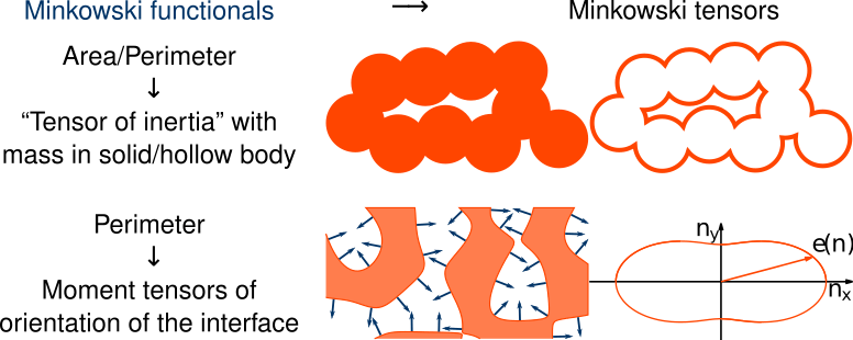
The scalar functionals can be interpreted as area, perimeter, or the Euler characteristic, which is a topological constant. The vectors are closely related to the centers of mass in either solid or hollow bodies. Accordingly, the second-rank tensors correspond the tensors of inertia, or they can be interpreted as the moment tensors of the distribution of the normals on the boundary.

Minkowski Functionals

Area
$W_0 = \quad \int\limits_K \mathrm d A \propto V_2$
Perimeter
$W_1 = \frac 12 \int\limits_{\partial K} \mathrm d l \propto V_1$
Euler characteristic
$W_2 = \frac 12 \int\limits_{\partial K} \kappa\, \mathrm d l \propto V_0$

with
$\kappa$ = curvature

2D-MF

Cartesian representation (Minkowski Tensors)

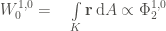
Using the position vector $\textbf r$ and the normal vector $\textbf n$ on the boundary, the Minkowski Vectors can be defined in the Cartesian representation.

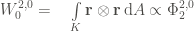
The second-rank Minkowski tensors are defined using the symmetric tensor product $(\textbf a\otimes \textbf a)_{ij} = a_i a_j$ .

Minkowski Vectors

$W_0^{1,0} = \quad \int\limits_K \textbf r \, \mathrm d A\propto \Phi_2^{1,0}$
$W_1^{1,0} = \frac 12 \int\limits_{\partial K} \textbf r \, \mathrm d l\propto \Phi_1^{1,0}$
$W_2^{1,0} = \frac 12 \int\limits_{\partial K} \kappa \, \textbf r \, \mathrm d l\propto \Phi_0^{1,0}$

Minkowski Tensors

$W_0^{2,0} = \quad \int\limits_K \textbf r \otimes \textbf r \, \mathrm d A\propto \Phi_2^{2,0}$
$W_1^{2,0} = \frac 12 \int\limits_{\partial K} \textbf r \otimes \textbf r \, \mathrm d l\propto \Phi_1^{2,0}$
$W_2^{2,0} = \frac 12 \int\limits_{\partial K} \kappa \, \textbf r \otimes \textbf r \, \mathrm d l\propto \Phi_0^{2,0}$
$W_1^{0,2} = \frac 12 \int\limits_{\partial K} \textbf n \otimes \textbf n \, \mathrm d l\propto \Phi_1^{0,2}$
$W_2^{0,2} = \frac 12 \int\limits_{\partial K} \kappa \, \textbf n \otimes \textbf n \, \mathrm d l\propto \Phi_0^{0,2}$

2D-MT

Irreducible representation (Circular Minkowski Tensors)

under construction

Consider a polygon with edges L:
$\vec L_i = L_i \cdot \vec n_i$

Density of normals:
$\rho(\varphi) = \sum L_i \delta(\phi-\phi_i)$

Fourier analysis:
$\tilde\rho(l) = \int \textnormal d \varphi \, \textnormal{exp}(i l \varphi) \, \rho(\varphi) = \sum L_i \textnormal{exp}(i l \varphi_i)$

$\tilde\rho(0) = L = W_1$ (the circumference of the polygon)
$\tilde\rho(1) = 0$ (for a closed polygon)

The shape indexes $q_l$ are defined as
$q_l = \frac{|\tilde\rho(l)|}{\tilde\rho(0)}$ .

$q_0$ is the circumference of the object.
$q_1 = 1$ for closed polygons.
$q_2$ is the polar component of the normal density, it is related to $\beta_1^{0,2} - 1$
$q_3$ can detect anisotropy in a three-fold symmetric system
$q_4$ is the quadrupole component (suitable for detecting rectangles)
$q_6$ : …